MMM Multidimensional Example Notebook#
In this notebook, we present an new experimental media mix model class to create multidimensional and customized marketing mix models. To showcase its capabilities, we extend the MMM Example Notebook simulation to create a multidimensional hierarchical model.
Warning
Even though the new MMM class is an experimental class, it is fully functional and can be used to create multidimensional marketing mix models. This model is under active development and will be further improved in the future (feedback welcome!).
Prepare Notebook#
import warnings

import arviz as az
import arviz_plots as azp
import matplotlib.pyplot as plt
import numpy as np
import pandas as pd
import pymc as pm
import seaborn as sns
import xarray as xr
from pymc_extras.prior import Prior

from pymc_marketing.mmm import GeometricAdstock, LogisticSaturation
from pymc_marketing.mmm.mmm import (
    MMM,
    BudgetOptimizerWrapper,
)
from pymc_marketing.paths import data_dir
from pymc_marketing.special_priors import LaplacePrior, LogNormalPrior

warnings.filterwarnings("ignore", category=UserWarning)

az.style.use("arviz-vibrant")
plt.rcParams["figure.figsize"] = [12, 7]
plt.rcParams["figure.dpi"] = 100
plt.rcParams["xtick.labelsize"] = 10
plt.rcParams["ytick.labelsize"] = 8

%load_ext autoreload
%autoreload 2
%config InlineBackend.figure_format = "retina"
seed: int = sum(map(ord, "mmm_multidimensional"))
rng: np.random.Generator = np.random.default_rng(seed=seed)
Read Data#
We read the simulated data from the MMM Multidimensional Example Notebook.
data_path = data_dir / "mmm_multidimensional_example.csv"

data_df = pd.read_csv(data_path, parse_dates=["date"])
data_df.info()
<class 'pandas.core.frame.DataFrame'>
RangeIndex: 318 entries, 0 to 317
Data columns (total 7 columns):
 #   Column   Non-Null Count  Dtype
---  ------   --------------  -----
 0   date     318 non-null    datetime64[ns]
 1   geo      318 non-null    object
 2   x1       318 non-null    float64
 3   x2       318 non-null    float64
 4   event_1  318 non-null    int64
 5   event_2  318 non-null    int64
 6   y        318 non-null    float64
dtypes: datetime64[ns](1), float64(3), int64(2), object(1)
memory usage: 17.5+ KB
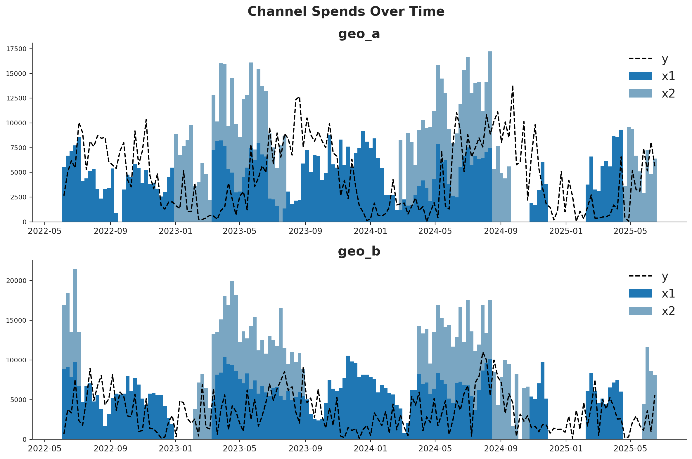
For our setup, imagine we are selling one product in two different countries (geo_a and geo_b). Our marketing team maintains two channels - one is a usually-on channel while the other channel is more tactical and is turned on during marketing campaigns. Visual inspection of the data suggests that there is at least some effect of marketing on sales, but the relationship is noisy. Our mission is to see if the MMM can parse the signal in the noise.
One strategy for dealing with noisy, low-signal data is to borrow information from similar contexts. If channel 2 seems to be pretty effective in geo_b, that gives us reason to suspect it will be effective in geo_a. This can be implemented either with full pooling or partial pooling (partial pooling models are often called ‘hierarchical’ or ‘multi-level’). So this notebook will demonstrate how to fit an MMM to multiple markets at the same time and make decisions about how to pool information across the two contexts.
fig, (ax1, ax2) = plt.subplots(2, 1, figsize=(12, 8))
fig.suptitle("Channel Spends Over Time", fontsize=16, fontweight="bold")

blue_colors = ["#1f77b4", "#7aa6c2"]  # Darker and lighter shades of blue

# Plot for geo_a
geo_a_data = data_df[data_df["geo"] == "geo_a"]
ax1.bar(geo_a_data["date"], geo_a_data["x1"], label="x1", width=7, color=blue_colors[0])
ax1.bar(
    geo_a_data["date"],
    geo_a_data["x2"],
    bottom=geo_a_data["x1"],
    label="x2",
    width=7,
    color=blue_colors[1],
)
ax1.plot(geo_a_data["date"], geo_a_data["y"], "--", label="y", color="black")
ax1.set_title("geo_a")
ax1.legend()

# Plot for geo_b
geo_b_data = data_df[data_df["geo"] == "geo_b"]
ax2.bar(geo_b_data["date"], geo_b_data["x1"], label="x1", width=7, color=blue_colors[0])
ax2.bar(
    geo_b_data["date"],
    geo_b_data["x2"],
    bottom=geo_b_data["x1"],
    label="x2",
    width=7,
    color=blue_colors[1],
)
ax2.plot(geo_b_data["date"], geo_b_data["y"], "--", label="y", color="black")
ax2.set_title("geo_b")
ax2.legend()

plt.tight_layout()
Prior Specification#
A product may perform very differently in distinct markets, popular in some locations but rather niche in others. If this is the case, observing how a product is doing in one market doesn’t tell us much about how it will be doing in another.
Alternatively, a product may behave very consistently across markets, either always loved or ignored. If so, we can better predict response across markets, including for those that we may only have noisy measurements.
More realistically, hierarchical models allow for a continuous interpolation between these two scenarios, adaptively pooling information to the extent it seems warranted. This is also called partial pooling. If you need an introduction on Bayesian hierarchical models, check out the comprehensive example “A Primer on Bayesian Methods for Multilevel Modeling” in the PyMC documentation.
This notebook we’ll illustrate hierarchical modeling in MMM models. This can be controlled via the dims argument of Prior objects used in model_config. We’ll show you how to code each type of assumption you might make (we aren’t recommending it as a good model!).
Let’s start with the beta parameter of the saturation curve, which represents the maximum number of weekly sales you could drive through a channel. It will be the only parameter we model hierarchically.
The beta_prior below has dimensions of channel and geo, meaning we will have one beta parameter per channel and per geographic market. The parameters, mu and std, also have a prior. But critically, they only have channel dimensions.
This forces the prior parameters to be shared across distinct geographies and, therefore, be compatible with all of them.
Specifically, the prior on mean captures what we expect each channel to do on average, without considering their variation on geography, while the prior on std represents how much the effect varies across geographies. std encodes the strength of “pooling”. If it’s large, channels are expected to vary widely, if it’s small they are expected to be similarly behaved.
Note that distinct channels are still independent. If we wanted, we could have pooled information across channels by using a single mean and std prior shared between all channels and geographies.
beta_prior = LogNormalPrior(
    mean=Prior("Gamma", mu=0.25, sigma=0.10, dims="channel"),
    std=Prior("Exponential", scale=0.10, dims="channel"),
    dims=("channel", "geo"),
    centered=False,
)
Next we look at lambda, which represents the efficiency of a channel. The higher the lambda, the faster sales respond to spending on that channel. We’ll have the lambda parameter be fully pooled across all geographies. We are assuming that channel 1 has the same efficiency in both geographical markets, so we do not specify “geo” dims.
Note that by using constants for the parameters, there’s no shared learnable priors (i.e., hierarchical structure). This is what enforces a complete pooling structure.
lam_prior = Prior("Gamma", mu=0.5, sigma=0.25, dims="channel")

saturation = LogisticSaturation(
    priors={
        "beta": beta_prior,
        "lam": lam_prior,
    },
)
saturation.model_config
{'saturation_lam': Prior("Gamma", mu=0.5, sigma=0.25, dims="channel"),
 'saturation_beta': <pymc_marketing.special_priors.LogNormalPrior at 0x1505a8c20>}
The alpha parameter of the Adstock function represents how long customers remember marketing. We’ll choose an unpooled structure. Here, each channel in each geography has its own effect and those effects do not influence each other. Notice that we put a dim for both geos and channels to indicate that we want 4 unique effects.
Once again we have no learnable parameters inside the prior of alpha. We could have tried to specify priors with the same dimensions geo and channel, which would still imply no-pooling of information. But if we did that, the model would become too undetermined, with each parameter prior only informed by one single alpha parameter each.
alpha_prior = Prior("Beta", alpha=2, beta=5, dims=("geo", "channel"))

adstock = GeometricAdstock(
    priors={"alpha": alpha_prior},
    l_max=8,
)

adstock.model_config
{'adstock_alpha': Prior("Beta", alpha=2, beta=5, dims=("geo", "channel"))}
You can mix and match the unpooled, fully pooled, and partially pooled strategy for any of your effects. You can extend this strategy to controls or noise parameters as well. Given the variety of options, it can be hard to know which pooling strategy to choose for a given effect. In our opinion, the choice is primarily driven by computational considerations. Partial pooling is generally a more reasonable assumption, but it can make the model slower or harder to estimate, and more difficult to reason about.
For example, you might notice that we set our beta prior with centered=False. This is known as a reparameterization, a strategy to solve computational difficulties that MCMC algorithms can run into when fitting hierarchical models, specially with small dimensions (remember we have just two channels and two geographies!).
We recommend that you start with a model that uses only fully pooled or unpooled effects. Once you have a good working model you can add complexity slowly, verifying your model performance and accuracy at each stage.
We complete the model specification with similar priors as in the MMM Example Notebook.
model_config = {
    "intercept": Prior("Gamma", mu=0.5, sigma=0.25, dims="geo"),
    "gamma_control": Prior("Normal", mu=0, sigma=0.5, dims="control"),
    "gamma_fourier": LaplacePrior(
        mu=0,
        b=Prior("HalfNormal", sigma=0.2),
        dims=("geo", "fourier_mode"),
        centered=False,
    ),
    "likelihood": Prior(
        "TruncatedNormal",
        lower=0,
        sigma=Prior("HalfNormal", sigma=1.5),
        dims=("date", "geo"),
    ),
}
Model Definition#
We are now ready to define the model class. The API is very similar to the one in the MMM Example Notebook.
# Base MMM model specification
mmm = MMM(
    date_column="date",
    target_column="y",
    channel_columns=["x1", "x2"],
    control_columns=["event_1", "event_2"],
    dims=("geo",),
    scaling={
        "channel": {"method": "max", "dims": ()},
        "target": {"method": "max", "dims": ()},
    },
    adstock=adstock,
    saturation=saturation,
    yearly_seasonality=2,
    model_config=model_config,
)
Tip
Observe we have the following two new arguments:
dims: a tuple of strings that specify the dimensions of the model.scaling: a dictionary that specifies the scaling method and dimensions for the target and media variables. In this case we leave the dimensions empty as we want to scale the target variable for each geo (see details below).
We can now prepare the training data.
x_train = data_df.drop(columns=["y"])
y_train = data_df["y"]
To build the model, we need to specify the training data and the target variables.
Tip
We do not need to build the model, we can simply fit the model. This is just to inspect the model structure.
mmm.build_model(X=x_train, y=y_train)
Let’s look into the model graph:
mmm.model.to_graphviz()

It may be easier to visualize the dimensions of each parameter in a table format:
mmm.table()
                             Variable  Expression                             Dimensions
───────────────────────────────────────────────────────────────────────────────────────────────────────────────────
                      channel_scale =  Data                                   geo[2] × channel[2]
                       target_scale =  Data                                   geo[2]
                       channel_data =  Data                                   date[159] × geo[2] × channel[2]
                        target_data =  Data                                   date[159] × geo[2]
                       control_data =  Data                                   date[159] × geo[2] × control[2]
                          dayofyear =  Data                                   date[159]

             intercept_contribution ~  Gamma(<constant>, <constant>)          geo[2]
                      adstock_alpha ~  Beta(2, 5)                             geo[2] × channel[2]
                     saturation_lam ~  Gamma(<constant>, <constant>)          channel[2]
               saturation_beta_mean ~  Gamma(<constant>, <constant>)          channel[2]
                saturation_beta_std ~  Exponential(0.1)                       channel[2]
         saturation_beta_log_offset ~  Normal(0, 1)                           channel[2] × geo[2]
                      gamma_control ~  Normal(0, 0.5)                         control[2]
                    gamma_fourier_b ~  HalfNormal(0, 0.2)
                gamma_fourier_sigma ~  Exponential(f(gamma_fourier_b))
               gamma_fourier_offset ~  Normal(0, 1)                           geo[2] × fourier_mode[4]
                            y_sigma ~  HalfNormal(0, 1.5)
                                                                              Parameter count = 29

                    saturation_beta =  f(saturation_beta_log_offset,          channel[2] × geo[2]
                                       saturation_beta_mean,
                                       saturation_beta_std)
               channel_contribution =  f(saturation_beta_log_offset,          date[159] × channel[2] × geo[2]
                                       saturation_lam, saturation_beta_mean,
                                       saturation_beta_std, adstock_alpha)
               control_contribution =  f(gamma_control)                       date[159] × geo[2] × control[2]
                      gamma_fourier =  f(gamma_fourier_offset,                geo[2] × fourier_mode[4]
                                       gamma_fourier_sigma)
               fourier_contribution =  f(gamma_fourier_offset,                date[159] × geo[2] × fourier_mode[4]
                                       gamma_fourier_sigma)
    yearly_seasonality_contribution =  f(gamma_fourier_offset,                date[159] × geo[2]
                                       gamma_fourier_sigma)
 total_media_contribution_original_s…  f(saturation_beta_log_offset,
                                    =  saturation_lam, saturation_beta_mean,
                                       saturation_beta_std, adstock_alpha)

                                  y ~  Unknown(TruncatedNormal(f(intercept_…  date[159] × geo[2]
                                       gamma_control, gamma_fourier_offset,
                                       gamma_fourier_sigma,
                                       saturation_beta_log_offset,
                                       saturation_lam, saturation_beta_mean,
                                       saturation_beta_std, adstock_alpha),
                                       y_sigma, 0, inf))
It is great to see that the model automatically vectorizes and creates the expected hierarchies and dimensions 🚀!
As we are scaling our data internally, we can add deterministic terms to recover the component contributions in the original scale.
mmm.add_original_scale_contribution_variable(
    var=[
        "channel_contribution",
        "control_contribution",
        "intercept_contribution",
        "yearly_seasonality_contribution",
        "y",
    ]
)

pm.model_to_graphviz(mmm.model)

Coming back to the scalers, we can get them as an xarray dataset.
scalers = mmm.get_scales_as_xarray()

scalers
{'channel_scale': <xarray.DataArray '_channel' (geo: 2, channel: 2)> Size: 32B
 array([[ 9318.97848455,  9755.9729876 ],
        [10555.0774866 , 11760.98180037]])
 Coordinates:
   * geo      (geo) object 16B 'geo_a' 'geo_b'
   * channel  (channel) object 16B 'x1' 'x2',
 'target_scale': <xarray.DataArray '_target' (geo: 2)> Size: 16B
 array([13812.08025674, 11002.97913936])
 Coordinates:
   * geo      (geo) object 16B 'geo_a' 'geo_b'}
As expected, from the model definition, we have scalers for the target and media variables across geos.
Prior Predictive Checks#
Before fitting the model, we can inspect the prior predictive distribution.
with mmm.model:
    prior = pm.sample_prior_predictive()
prior
/Users/will/github/pymc-eco/pymc-marketing/worktrees/pymc6-migrate/.venv/lib/python3.13/site-packages/pytensor/assumptions/diagonal.py:53: RuntimeWarning: invalid value encountered in multiply
  result = FactState.FALSE if np.any(data * ~eye_mask) else FactState.TRUE
Sampling: [adstock_alpha, gamma_control, gamma_fourier_b, gamma_fourier_offset, gamma_fourier_sigma, intercept_contribution, saturation_beta_log_offset, saturation_beta_mean, saturation_beta_std, saturation_lam, y, y_sigma]
<xarray.DataTree>
Group: /
├── Group: /prior
│       Dimensions:                                         (chain: 1, draw: 500,
│                                                            date: 159, geo: 2,
│                                                            control: 2, channel: 2,
│                                                            fourier_mode: 4)
│       Coordinates:
│         * chain                                           (chain) int64 8B 0
│         * draw                                            (draw) int64 4kB 0 1 ... 499
│         * date                                            (date) datetime64[ns] 1kB ...
│         * geo                                             (geo) <U5 40B 'geo_a' 'ge...
│         * control                                         (control) <U7 56B 'event_...
│         * channel                                         (channel) <U2 16B 'x1' 'x2'
│         * fourier_mode                                    (fourier_mode) <U5 80B 's...
│       Data variables: (12/23)
│           yearly_seasonality_contribution_original_scale  (chain, draw, date, geo) float64 1MB ...
│           y_sigma                                         (chain, draw) float64 4kB ...
│           control_contribution_original_scale             (chain, draw, date, geo, control) float64 3MB ...
│           saturation_lam                                  (chain, draw, channel) float64 8kB ...
│           saturation_beta_std                             (chain, draw, channel) float64 8kB ...
│           y_original_scale                                (chain, draw, date, geo) float64 1MB ...
│           ...                                              ...
│           channel_contribution_original_scale             (chain, draw, date, channel, geo) float64 3MB ...
│           intercept_contribution_original_scale           (chain, draw, geo) float64 8kB ...
│           intercept_contribution                          (chain, draw, geo) float64 8kB ...
│           channel_contribution                            (chain, draw, date, channel, geo) float64 3MB ...
│           gamma_control                                   (chain, draw, control) float64 8kB ...
│           fourier_contribution                            (chain, draw, date, geo, fourier_mode) float64 5MB ...
│       Attributes:
│           created_at:                 2026-06-09T23:56:45.240157+00:00
│           creation_library:           ArviZ
│           creation_library_version:   1.1.0
│           creation_library_language:  Python
│           inference_library:          pymc
│           inference_library_version:  6.0.1
│           sample_dims:                ['chain', 'draw']
├── Group: /prior_predictive
│       Dimensions:  (chain: 1, draw: 500, date: 159, geo: 2)
│       Coordinates:
│         * chain    (chain) int64 8B 0
│         * draw     (draw) int64 4kB 0 1 2 3 4 5 6 7 ... 493 494 495 496 497 498 499
│         * date     (date) datetime64[ns] 1kB 2022-06-06 2022-06-13 ... 2025-06-16
│         * geo      (geo) <U5 40B 'geo_a' 'geo_b'
│       Data variables:
│           y        (chain, draw, date, geo) float64 1MB 0.2265 2.307 ... 1.904 0.2087
│       Attributes:
│           created_at:                 2026-06-09T23:56:45.244523+00:00
│           creation_library:           ArviZ
│           creation_library_version:   1.1.0
│           creation_library_language:  Python
│           inference_library:          pymc
│           inference_library_version:  6.0.1
│           sample_dims:                ['chain', 'draw']
├── Group: /observed_data
│       Dimensions:  (date: 159, geo: 2)
│       Coordinates:
│         * date     (date) datetime64[ns] 1kB 2022-06-06 2022-06-13 ... 2025-06-16
│         * geo      (geo) <U5 40B 'geo_a' 'geo_b'
│       Data variables:
│           y        (date, geo) float64 3kB 0.1917 0.06202 0.3635 ... 0.4068 0.5073
│       Attributes:
│           created_at:                 2026-06-09T23:56:45.245284+00:00
│           creation_library:           ArviZ
│           creation_library_version:   1.1.0
│           creation_library_language:  Python
│           inference_library:          pymc
│           inference_library_version:  6.0.1
│           sample_dims:                []
└── Group: /constant_data
        Dimensions:        (geo: 2, channel: 2, date: 159, control: 2)
        Coordinates:
          * geo            (geo) <U5 40B 'geo_a' 'geo_b'
          * channel        (channel) <U2 16B 'x1' 'x2'
          * date           (date) datetime64[ns] 1kB 2022-06-06 ... 2025-06-16
          * control        (control) <U7 56B 'event_1' 'event_2'
        Data variables:
            channel_scale  (geo, channel) float64 32B 9.319e+03 9.756e+03 ... 1.176e+04
            target_scale   (geo) float64 16B 1.381e+04 1.1e+04
            channel_data   (date, geo, channel) float64 5kB 5.528e+03 0.0 ... 8.091e+03
            target_data    (date, geo) float64 3kB 2.648e+03 682.4 ... 5.581e+03
            control_data   (date, geo, control) int64 5kB 0 0 0 0 0 0 0 ... 0 0 0 0 0 0
            dayofyear      (date) int32 636B 157 164 171 178 185 ... 139 146 153 160 167
        Attributes:
            created_at:                 2026-06-09T23:56:45.247773+00:00
            creation_library:           ArviZ
            creation_library_version:   1.1.0
            creation_library_language:  Python
            inference_library:          pymc
            inference_library_version:  6.0.1
sample_dims: []g = sns.relplot(
data=data_df,
x="date",
y="y",
color="black",
col="geo",
col_wrap=1,
kind="line",
height=4,
aspect=3,
)
axes = g.axes.flatten()
for ax, geo in zip(axes, mmm.model.coords["geo"], strict=True):
hdi = az.hdi(
prior.prior.sel(geo=geo)
.dataset["y_original_scale"]
.unstack()
.transpose(..., "date"),
prob=0.94,
)
ax.fill_between(
mmm.model.coords["date"],
hdi.sel(ci_bound="lower"),
hdi.sel(ci_bound="upper"),
color="C0",
alpha=0.3,
label="94% HDI",
)
hdi = az.hdi(
prior.prior.sel(geo=geo)
.dataset["y_original_scale"]
.unstack()
.transpose(..., "date"),
prob=0.5,
)
ax.fill_between(
mmm.model.coords["date"],
hdi.sel(ci_bound="lower"),
hdi.sel(ci_bound="upper"),
color="C0",
alpha=0.5,
label="50% HDI",
)
ax.legend(loc="upper left")
g.figure.suptitle("Prior Predictive", fontsize=16, fontweight="bold", y=1.03);
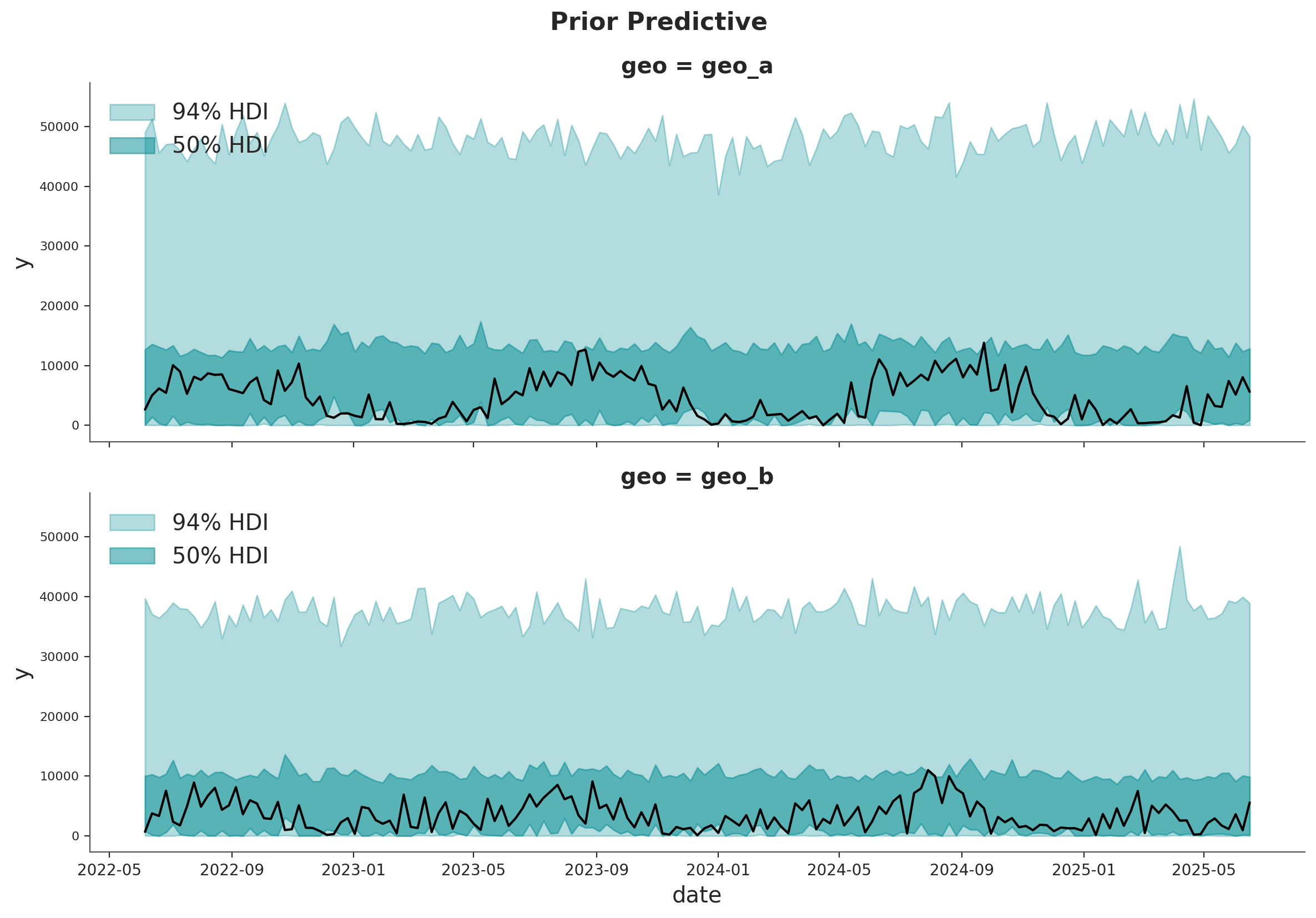
The prior predictive distribution looks good and not too restrictive.
Model Fitting#
We can now fit the model and generate the posterior predictive distribution.
mmm.fit(
    X=x_train,
    y=y_train,
    chains=4,
    target_accept=0.95,
    random_seed=rng,
)

mmm.sample_posterior_predictive(
    X=x_train,
    random_seed=rng,
)
/Users/will/github/pymc-eco/pymc-marketing/worktrees/pymc6-migrate/.venv/lib/python3.13/site-packages/pytensor/assumptions/diagonal.py:53: RuntimeWarning: invalid value encountered in multiply
  result = FactState.FALSE if np.any(data * ~eye_mask) else FactState.TRUE
NUTS[nutpie]: [y_sigma, gamma_fourier_b, gamma_fourier_sigma, gamma_fourier_offset, gamma_control, adstock_alpha, saturation_lam, saturation_beta_mean, saturation_beta_std, saturation_beta_log_offset, intercept_contribution]
/Users/will/github/pymc-eco/pymc-marketing/worktrees/pymc6-migrate/.venv/lib/python3.13/site-packages/pytensor/assumptions/diagonal.py:53: RuntimeWarning: invalid value encountered in multiply
  result = FactState.FALSE if np.any(data * ~eye_mask) else FactState.TRUE
/Users/will/github/pymc-eco/pymc-marketing/worktrees/pymc6-migrate/.venv/lib/python3.13/site-packages/pytensor/assumptions/diagonal.py:53: RuntimeWarning: invalid value encountered in multiply
  result = FactState.FALSE if np.any(data * ~eye_mask) else FactState.TRUE
/Users/will/github/pymc-eco/pymc-marketing/worktrees/pymc6-migrate/.venv/lib/python3.13/site-packages/pytensor/assumptions/diagonal.py:53: RuntimeWarning: invalid value encountered in multiply
  result = FactState.FALSE if np.any(data * ~eye_mask) else FactState.TRUE
Sampling: [y]
<xarray.Dataset> Size: 20MB
Dimensions:           (date: 159, geo: 2, sample: 4000)
Coordinates:
  * date              (date) datetime64[ns] 1kB 2022-06-06 ... 2025-06-16
  * geo               (geo) <U5 40B 'geo_a' 'geo_b'
  * sample            (sample) object 32kB MultiIndex
  * chain             (sample) int64 32kB 0 0 0 0 0 0 0 0 0 ... 3 3 3 3 3 3 3 3
  * draw              (sample) int64 32kB 0 1 2 3 4 5 ... 995 996 997 998 999
Data variables:
    y                 (date, geo, sample) float64 10MB 0.504 0.5833 ... 0.032
    y_original_scale  (date, geo, sample) float64 10MB 6.961e+03 ... 352.1
Attributes:
    created_at:                 2026-06-09T23:57:03.477445+00:00
    creation_library:           ArviZ
    creation_library_version:   1.1.0
    creation_library_language:  Python
    inference_library:          pymc
    inference_library_version:  6.0.1
sample_dims: ['sample']The sampling looks good. No divergences and the r-hat values are close to \(1\).
mmm.idata.sample_stats.diverging.sum("draw")
<xarray.DataArray 'diverging' (chain: 4)> Size: 32B
array([0, 0, 0, 0])
Coordinates:
  * chain    (chain) int64 32B 0 1 2 3
az.summary(
    mmm.idata,
    var_names=[
        "adstock_alpha",
        "gamma_control",
        "gamma_fourier",
        "intercept_contribution",
        "saturation_beta",
        "saturation_beta_mean",
        "saturation_beta_std",
        "saturation_lam",
        "y_sigma",
    ],
)
| mean | sd | eti89_lb | eti89_ub | ess_bulk | ess_tail | r_hat | mcse_mean | mcse_sd | |
|---|---|---|---|---|---|---|---|---|---|
| adstock_alpha[geo_a, x1] | 0.295 | 0.158 | 0.075 | 0.58 | 5881 | 2584 | 1.00 | 0.002 | 0.0014 |
| adstock_alpha[geo_a, x2] | 0.31 | 0.166 | 0.075 | 0.61 | 6057 | 2355 | 1.00 | 0.002 | 0.0014 |
| adstock_alpha[geo_b, x1] | 0.264 | 0.153 | 0.058 | 0.54 | 5570 | 2348 | 1.00 | 0.0019 | 0.0014 |
| adstock_alpha[geo_b, x2] | 0.279 | 0.165 | 0.059 | 0.58 | 6571 | 2472 | 1.00 | 0.002 | 0.0013 |
| gamma_control[event_1] | 0.302 | 0.085 | 0.17 | 0.44 | 6209 | 3584 | 1.00 | 0.0011 | 0.00075 |
| gamma_control[event_2] | -0.099 | 0.093 | -0.25 | 0.045 | 6531 | 3047 | 1.00 | 0.0012 | 0.00085 |
| gamma_fourier[geo_a, sin_1] | -0.35 | 0.0359 | -0.41 | -0.29 | 3578 | 3130 | 1.00 | 0.00061 | 0.00044 |
| gamma_fourier[geo_a, sin_2] | -0.0285 | 0.0284 | -0.074 | 0.016 | 4207 | 3038 | 1.00 | 0.00044 | 0.00032 |
| gamma_fourier[geo_a, cos_1] | -0.286 | 0.0333 | -0.34 | -0.24 | 4446 | 3653 | 1.00 | 0.0005 | 0.00039 |
| gamma_fourier[geo_a, cos_2] | 0.0045 | 0.0273 | -0.038 | 0.049 | 5661 | 3006 | 1.00 | 0.00036 | 0.00026 |
| gamma_fourier[geo_b, sin_1] | -0.0456 | 0.0251 | -0.086 | -0.0056 | 5501 | 3296 | 1.00 | 0.00034 | 0.00023 |
| gamma_fourier[geo_b, sin_2] | 0.19 | 0.0267 | 0.15 | 0.23 | 5326 | 3593 | 1.00 | 0.00037 | 0.00026 |
| gamma_fourier[geo_b, cos_1] | -0.1998 | 0.0299 | -0.25 | -0.15 | 5756 | 3638 | 1.00 | 0.00039 | 0.00028 |
| gamma_fourier[geo_b, cos_2] | -0.0292 | 0.0256 | -0.07 | 0.012 | 5767 | 3138 | 1.00 | 0.00034 | 0.00025 |
| intercept_contribution[geo_a] | 0.198 | 0.0298 | 0.15 | 0.24 | 2829 | 2330 | 1.00 | 0.00057 | 0.00039 |
| intercept_contribution[geo_b] | 0.213 | 0.0286 | 0.17 | 0.26 | 2772 | 2191 | 1.00 | 0.00056 | 0.00042 |
| saturation_beta[x1, geo_a] | 0.2 | 0.115 | 0.042 | 0.4 | 4044 | 3195 | 1.00 | 0.0018 | 0.0016 |
| saturation_beta[x1, geo_b] | 0.237 | 0.122 | 0.064 | 0.44 | 4665 | 3081 | 1.00 | 0.0018 | 0.002 |
| saturation_beta[x2, geo_a] | 0.274 | 0.17 | 0.08 | 0.53 | 3261 | 3009 | 1.00 | 0.0032 | 0.0082 |
| saturation_beta[x2, geo_b] | 0.239 | 0.126 | 0.067 | 0.45 | 4132 | 3230 | 1.00 | 0.0019 | 0.0026 |
| saturation_beta_mean[x1] | 0.24 | 0.09 | 0.12 | 0.4 | 4930 | 2814 | 1.00 | 0.0013 | 0.0011 |
| saturation_beta_mean[x2] | 0.247 | 0.091 | 0.12 | 0.41 | 4546 | 2901 | 1.00 | 0.0013 | 0.001 |
| saturation_beta_std[x1] | 0.108 | 0.105 | 0.0065 | 0.3 | 2877 | 2101 | 1.00 | 0.0016 | 0.0023 |
| saturation_beta_std[x2] | 0.092 | 0.095 | 0.0049 | 0.27 | 3814 | 2142 | 1.00 | 0.0013 | 0.0019 |
| saturation_lam[x1] | 0.472 | 0.221 | 0.18 | 0.86 | 3567 | 2810 | 1.00 | 0.0035 | 0.0032 |
| saturation_lam[x2] | 0.476 | 0.22 | 0.18 | 0.87 | 4587 | 2552 | 1.00 | 0.0031 | 0.0028 |
| y_sigma | 0.1837 | 0.0106 | 0.17 | 0.2 | 3690 | 3005 | 1.00 | 0.00018 | 0.00014 |
fig = plt.figure(figsize=(15, 15), layout="constrained")
azp.plot_trace(
    mmm.idata,
    var_names=[
        "adstock_alpha",
        "gamma_control",
        "gamma_fourier",
        "intercept_contribution",
        "saturation_beta",
        "saturation_beta_mean",
        "saturation_beta_std",
        "saturation_lam",
        "y_sigma",
    ],
)
fig.suptitle("Model Trace", fontsize=16, fontweight="bold", y=1.03)
plt.gcf().suptitle("Model Trace", fontsize=16, fontweight="bold", y=1.03);
---------------------------------------------------------------------------
ValueError                                Traceback (most recent call last)
Cell In[21], line 2
      1 fig = plt.figure(figsize=(15, 15), layout="constrained")
----> 2 azp.plot_trace(mmm.idata, var_names=["adstock_alpha", "gamma_control", "gamma_fourier", "intercept_contribution", "saturation_beta", "saturation_beta_mean", "saturation_beta_std", "saturation_lam", "y_sigma"], figure=fig)
      3 fig.suptitle("Model Trace", fontsize=16, fontweight="bold", y=1.03)
      4 plt.gcf().suptitle("Model Trace", fontsize=16, fontweight="bold", y=1.03);

File ~/github/pymc-eco/pymc-marketing/worktrees/pymc6-migrate/.venv/lib/python3.13/site-packages/arviz_plots/plots/trace_plot.py:141, in plot_trace(dt, var_names, filter_vars, group, coords, sample_dims, plot_collection, backend, labeller, aes_by_visuals, visuals, **pc_kwargs)
    139     pc_kwargs = set_wrap_layout(pc_kwargs, plot_bknd, distribution)
    140     pc_kwargs["figure_kwargs"].setdefault("sharex", True)
--> 141     plot_collection = PlotCollection.wrap(
    142         distribution,
    143         backend=backend,
    144         **pc_kwargs,
    145     )
    146 else:
    147     aux_dim_list = list(plot_collection.viz["plot"].dims)

File ~/github/pymc-eco/pymc-marketing/worktrees/pymc6-migrate/.venv/lib/python3.13/site-packages/arviz_plots/plot_collection.py:895, in PlotCollection.wrap(cls, data, cols, col_wrap, backend, figure_kwargs, **kwargs)
    888         viz_dict["col_index"][var_name] = aux_ds["col_index"]
    889 viz_dt = xr.DataTree(
    890     viz_dict["/"],
    891     children={
    892         key: xr.DataTree(xr.Dataset(value)) for key, value in viz_dict.items() if key != "/"
    893     },
    894 )
--> 895 return cls(data, viz_dt, backend=backend, **kwargs)

File ~/github/pymc-eco/pymc-marketing/worktrees/pymc6-migrate/.venv/lib/python3.13/site-packages/arviz_plots/plot_collection.py:268, in PlotCollection.__init__(self, data, viz_dt, aes_dt, aes, backend, **kwargs)
    266     if aes is None:
    267         aes = {}
--> 268     self._aes_dt = self.generate_aes_dt(aes, data, **kwargs)
    269 else:
    270     self._aes_dt = aes_dt

File ~/github/pymc-eco/pymc-marketing/worktrees/pymc6-migrate/.venv/lib/python3.13/site-packages/arviz_plots/plot_collection.py:542, in PlotCollection.generate_aes_dt(self, aes, data, **kwargs)
    540 extra_keys = [key for key in kwargs if key not in aes]
    541 if extra_keys:
--> 542     raise ValueError(
    543         f"Keyword arguments {extra_keys} have been passed as **kwargs but "
    544         "have no active aesthetic mapped to them. Keyword arguments must define "
    545         "values to use in their respective aesthetic mapping."
    546     )
    547 if not hasattr(self, "backend"):
    548     plot_bknd = import_module(".backend.none", package="arviz_plots")

ValueError: Keyword arguments ['figure'] have been passed as **kwargs but have no active aesthetic mapped to them. Keyword arguments must define values to use in their respective aesthetic mapping.
<Figure size 1500x1500 with 0 Axes>
Posterior Predictive Checks#
We can now inspect the posterior predictive distribution. As before, we need to scale the posterior predictive to the original scale to make it comparable to the data.
fig, axes = plt.subplots(
    nrows=len(mmm.model.coords["geo"]),
    figsize=(12, 9),
    sharex=True,
    sharey=True,
    layout="constrained",
)

for i, geo in enumerate(mmm.model.coords["geo"]):
    ax = axes[i]
    hdi = az.hdi(
        mmm.idata["posterior_predictive"].y_original_scale.sel(geo=geo), prob=0.94
    )
    ax.fill_between(
        mmm.model.coords["date"],
        hdi.sel(ci_bound="lower"),
        hdi.sel(ci_bound="upper"),
        color="C0",
        alpha=0.2,
        label="94% HDI",
    )
    hdi = az.hdi(
        mmm.idata["posterior_predictive"].y_original_scale.sel(geo=geo), prob=0.5
    )
    ax.fill_between(
        mmm.model.coords["date"],
        hdi.sel(ci_bound="lower"),
        hdi.sel(ci_bound="upper"),
        color="C0",
        alpha=0.4,
        label="50% HDI",
    )

    sns.lineplot(
        data=data_df.query("geo == @geo"),
        x="date",
        y="y",
        color="black",
        ax=ax,
    )

    ax.legend(loc="upper left")
    ax.set(title=f"{geo}")

fig.suptitle("Posterior Predictive", fontsize=16, fontweight="bold", y=1.03);
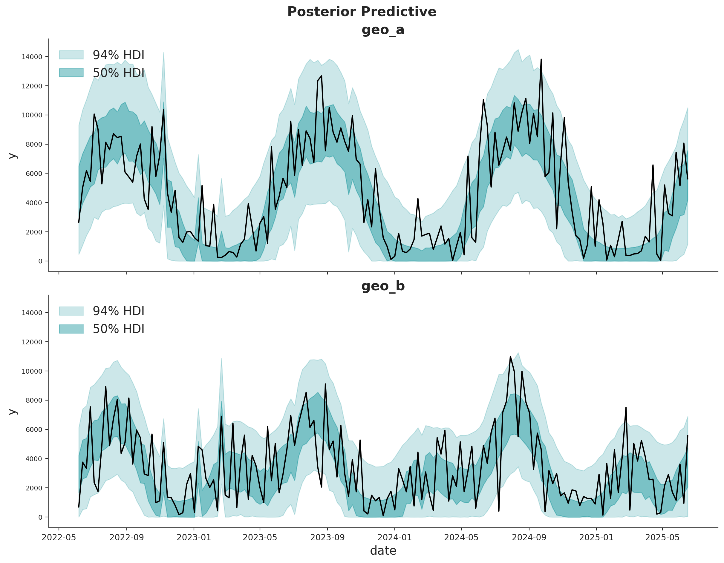
The fit looks okay! There is a lot of white-noise in the sales process we cannot predict. However, the main movements in the sales are either captured by our seasonality model or the MMM components.
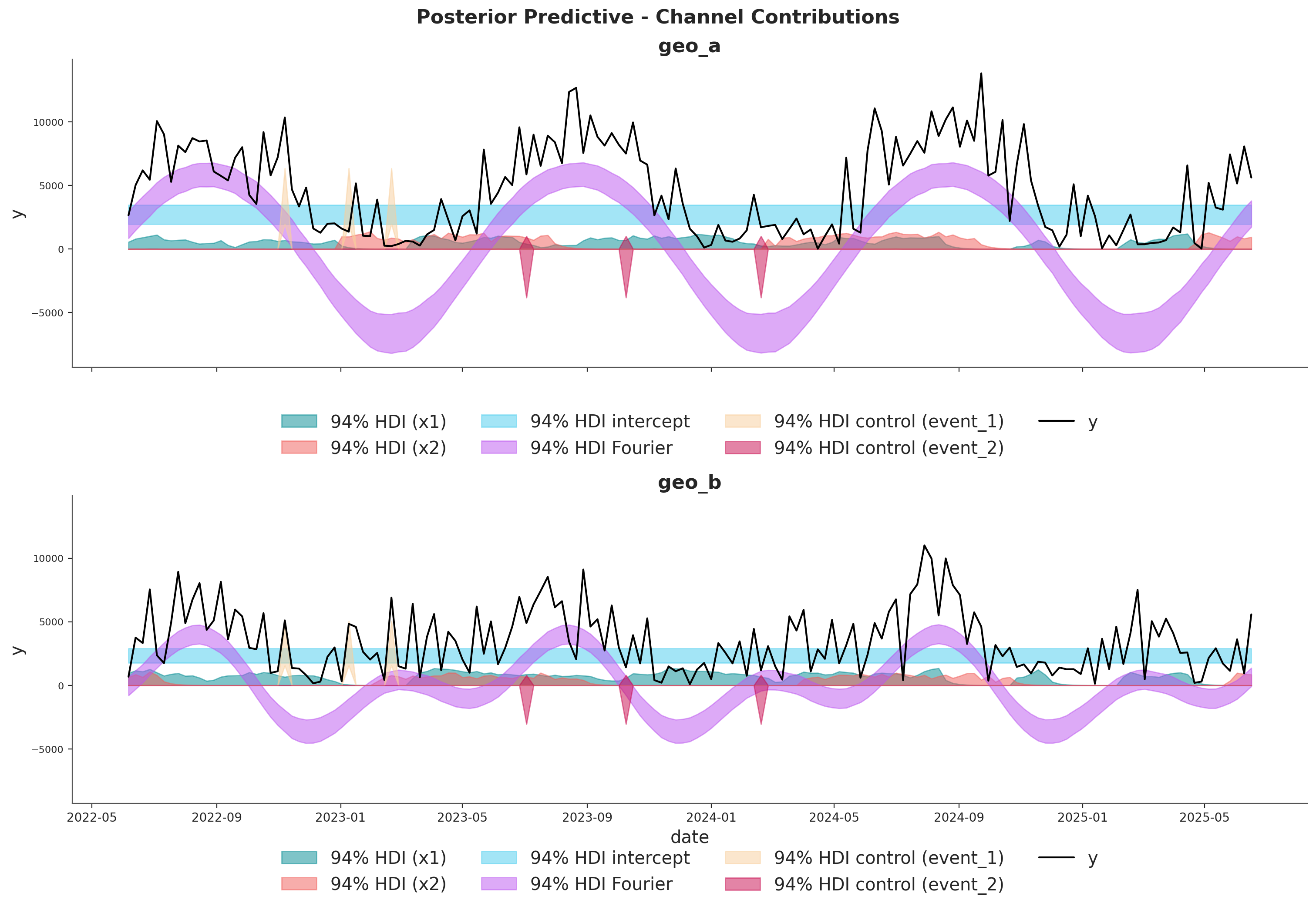
Model Components#
We can extract the contributions of each component of the model in the original scale thanks to the deterministic variables added to the model.
fig, axes = plt.subplots(
    nrows=len(mmm.model.coords["geo"]),
    figsize=(15, 10),
    sharex=True,
    sharey=True,
    layout="constrained",
)

for i, geo in enumerate(mmm.model.coords["geo"]):
    ax = axes[i]

    for j, channel in enumerate(mmm.model.coords["channel"]):
        hdi = az.hdi(
            mmm.idata["posterior"]["channel_contribution_original_scale"].sel(
                geo=geo, channel=channel
            ),
            prob=0.94,
        )
        ax.fill_between(
            mmm.model.coords["date"],
            hdi.sel(ci_bound="lower"),
            hdi.sel(ci_bound="upper"),
            color=f"C{j}",
            alpha=0.5,
            label=f"94% HDI ({channel})",
        )

    hdi = az.hdi(
        mmm.idata["posterior"]["intercept_contribution_original_scale"]
        .sel(geo=geo)
        .expand_dims({"date": mmm.model.coords["date"]})
        .transpose(..., "date"),
        prob=0.94,
    )
    ax.fill_between(
        mmm.model.coords["date"],
        hdi.sel(ci_bound="lower"),
        hdi.sel(ci_bound="upper"),
        color="C2",
        alpha=0.5,
        label="94% HDI intercept",
    )

    hdi = az.hdi(
        mmm.idata["posterior"]["yearly_seasonality_contribution_original_scale"].sel(
            geo=geo
        ),
        prob=0.94,
    )
    ax.fill_between(
        mmm.model.coords["date"],
        hdi.sel(ci_bound="lower"),
        hdi.sel(ci_bound="upper"),
        color="C3",
        alpha=0.5,
        label="94% HDI Fourier",
    )

    for k, control in enumerate(mmm.model.coords["control"]):
        hdi = az.hdi(
            mmm.idata["posterior"]["control_contribution_original_scale"].sel(
                geo=geo, control=control
            ),
            prob=0.94,
        )
        ax.fill_between(
            mmm.model.coords["date"],
            hdi.sel(ci_bound="lower"),
            hdi.sel(ci_bound="upper"),
            color=f"C{5 + k}",
            alpha=0.5,
            label=f"94% HDI control ({control})",
        )

    sns.lineplot(
        data=data_df.query("geo == @geo"),
        x="date",
        y="y",
        color="black",
        label="y",
        ax=ax,
    )
    ax.legend(
        loc="upper center",
        bbox_to_anchor=(0.5, -0.1),
        ncol=4,
    )
    ax.set(title=f"{geo}")

fig.suptitle(
    "Posterior Predictive - Channel Contributions",
    fontsize=16,
    fontweight="bold",
    y=1.03,
);
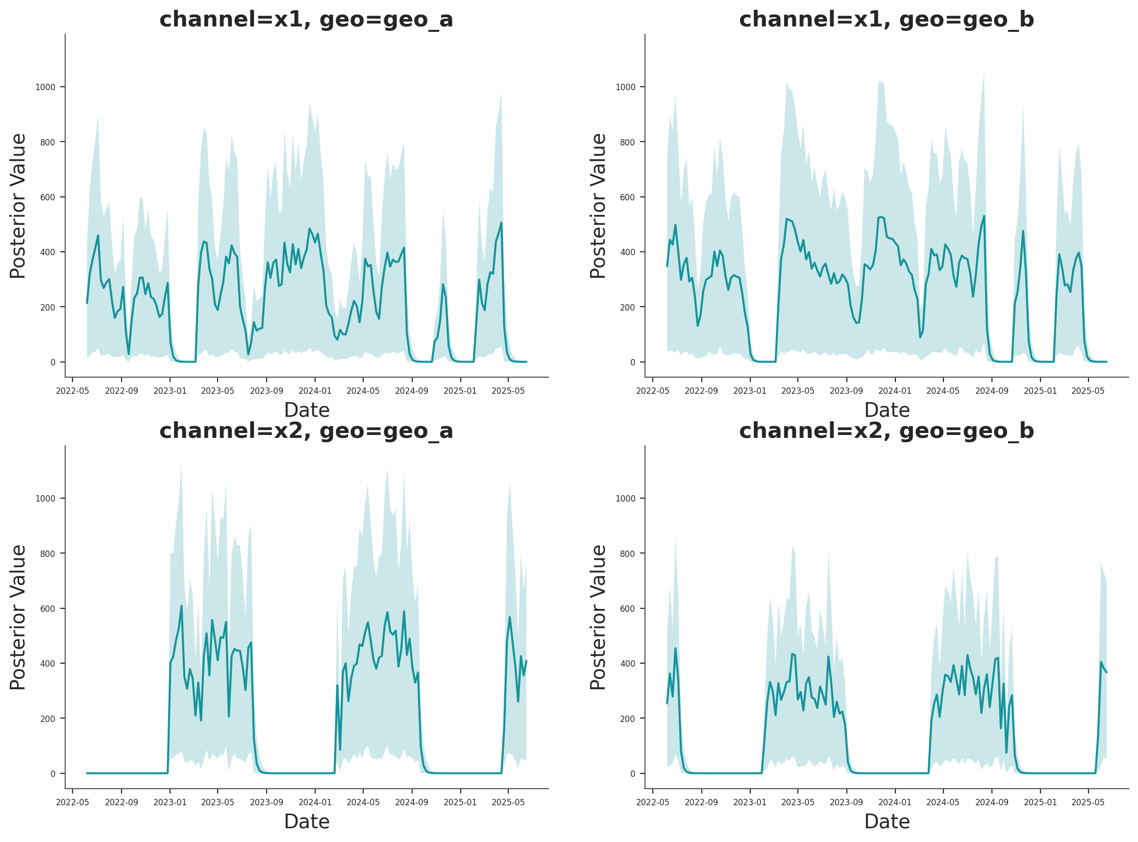
Media Deep Dive#
Next, we can look into the individual channel contributions across geos. This new class has a new plot name space that contains many plotting methods.
fig, axes = mmm.plot.contributions_over_time(
    var=["channel_contribution_original_scale"],
)

# Adjust figure size and layout to 2x2
fig.set_size_inches(14, 10)
fig.set_constrained_layout(True)

# Reshape axes to 2x2 grid
num_axes = len(axes.flatten())
if num_axes > 0:
    # Create a new 2x2 grid
    gs = fig.add_gridspec(2, 2)

    # Move existing axes to the new grid
    for i, ax in enumerate(axes.flatten()):
        if i < 4:  # Only handle up to 4 axes for 2x2 grid
            ax.set_position(gs[i // 2, i % 2].get_position(fig))

axes = axes.flatten()

# Share x and y axes across all subplots
for ax in axes:
    ax.legend().remove()
    ax.tick_params(axis="both", which="major", labelsize=6)
    ax.tick_params(axis="both", which="minor", labelsize=6)

# Share y axis limits
y_min = min(ax.get_ylim()[0] for ax in axes)
y_max = max(ax.get_ylim()[1] for ax in axes)
for ax in axes:
    ax.set_ylim(y_min, y_max)

# Share x axis limits
x_min = min(ax.get_xlim()[0] for ax in axes)
x_max = max(ax.get_xlim()[1] for ax in axes)
for ax in axes:
    ax.set_xlim(x_min, x_max)
/var/folders/v2/k_5glrgn4mbbh_g0l7zd21b00000gn/T/ipykernel_59800/2472926291.py:1: FutureWarning: The legacy MMMPlotSuite will be removed in pymc-marketing 2.0.0. Set mmm.plot_suite = 'new' to opt in to the new namespace-based API. See the migration guide: https://www.pymc-marketing.io/en/stable/notebooks/mmm/mmm_plot_suite_migration_guide.html
  fig, axes = mmm.plot.contributions_over_time(
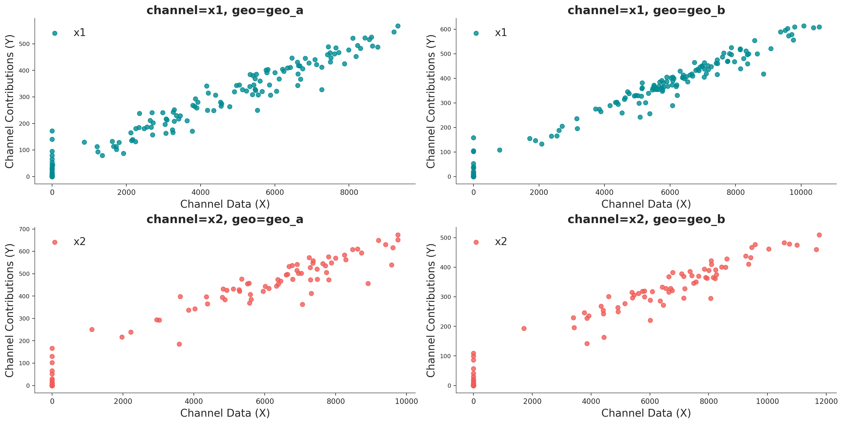
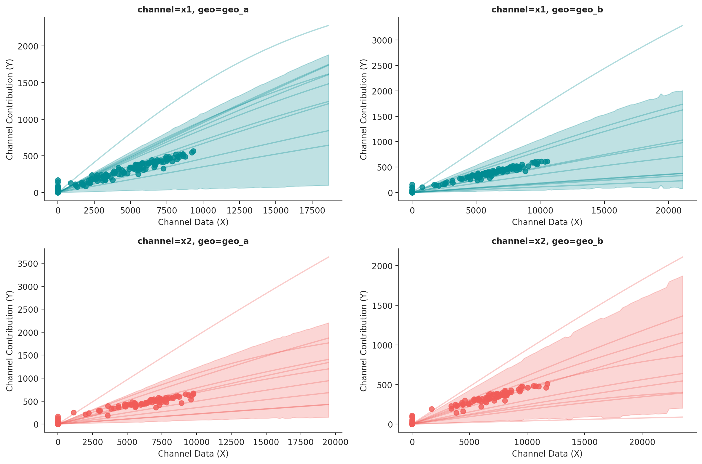
We can plot the saturation curves for each channel and geo, using a few different functions:
Using
saturation_scatterplot, we can get only the scatterplot between investment and estimated returns.Using
saturation_curves, we can get the posterior of the curves and their posterior fit regarding the given mean contribution.
mmm.plot.saturation_scatterplot(width_per_col=8, height_per_row=4, original_scale=True);
curve = mmm.saturation.sample_curve(mmm.idata.posterior, max_value=2)
fig, axes = mmm.plot.saturation_curves(
    curve,
    original_scale=True,
    n_samples=10,
    hdi_probs=0.85,
    random_seed=rng,
    subplot_kwargs={"figsize": (12, 8), "ncols": 2},
    rc_params={
        "xtick.labelsize": 10,
        "ytick.labelsize": 10,
        "axes.labelsize": 10,
        "axes.titlesize": 10,
    },
)

for ax in axes.ravel():
    ax.title.set_fontsize(10)

if fig._suptitle is not None:
    fig._suptitle.set_fontsize(12)

plt.tight_layout()
plt.show()
Sampling: []
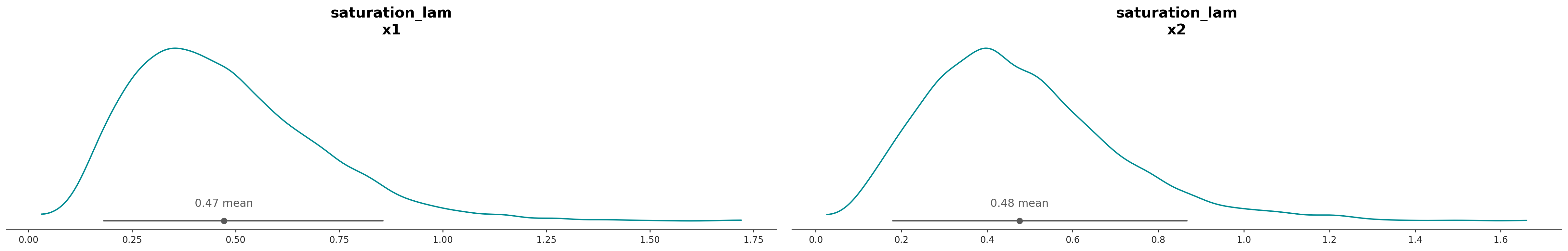
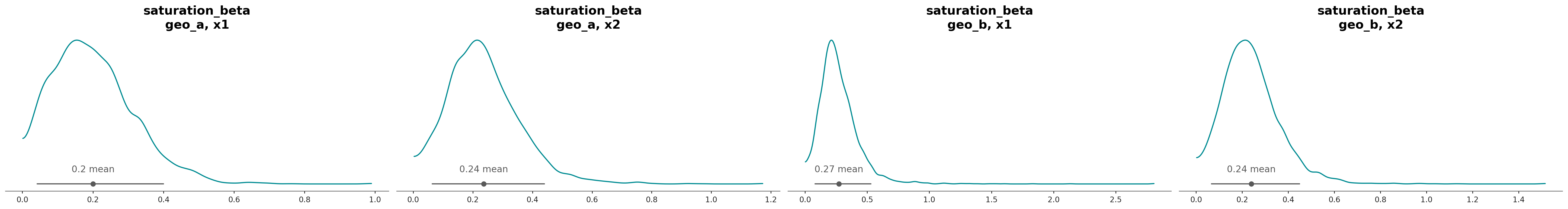
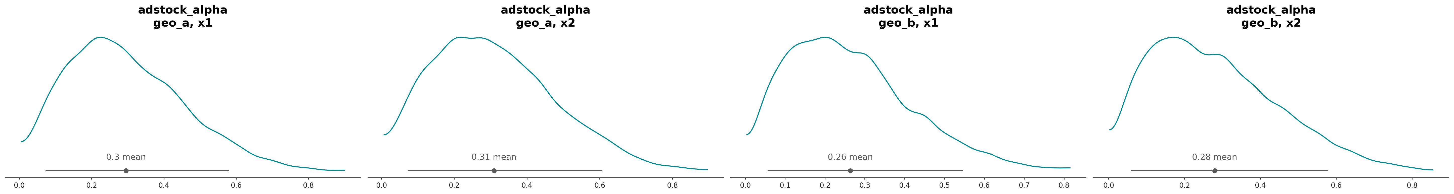
Parameter recovery#
One nice sign that the model is working as intend is that it can recover the true parameter values underlying the marketing mechanism. In our case, we know the true parameter values because we simulated the date. Informally, if the bulk of the posterior distribution covers the parameter value, that’s a good sign. We do not expect the mean of the posterior to always line up with the true value - for small or noisy data, we should expect the posterior to cover a wide interval regardless of whether we built a good model or not. There are also formal frameworks for thinking about parameter recovery in simulations that might be helpful if you need even more rigorous evidence the model is working correctly.
Below we compare the posterior distribution to the true values for the main MMM parameters (saturation lambda, saturation beta and adstock alpha).
# Load the true parameters used to generate the data

data_path = data_dir / "mmm_multidimensional_example_true_parameters.nc"
true_parameters = xr.open_dataset(data_path)
azp.plot_dist(
    xr.Dataset({"saturation_lam": mmm.fit_result["saturation_lam"]}),
);
azp.plot_dist(
    xr.Dataset({"saturation_beta": mmm.fit_result["saturation_beta"]}),
);
azp.plot_dist(
    xr.Dataset({"adstock_alpha": mmm.fit_result["adstock_alpha"]}),
);
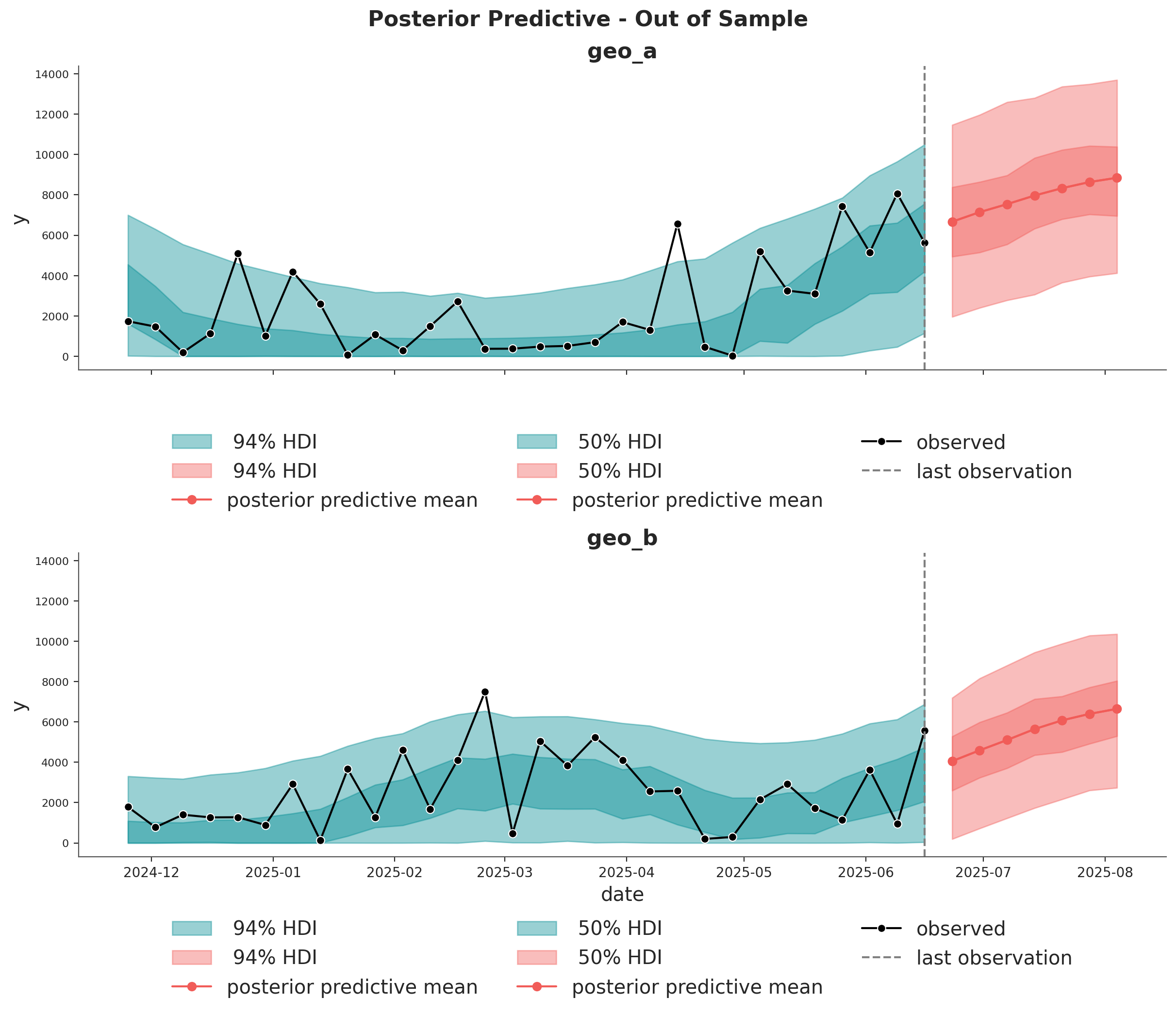
Out of Sample Predictions#
It is very important to be able to make predictions out of the sample. This is key for model validation, forward looking scenario planning and business decision making. Similarly as in the MMM Example Notebook, we assume the future spends are the same as the last day in the training sample. This way we can create a new dataset with the future dates and channel spends and use the model to make predictions.
last_date = x_train["date"].max()

# New dates starting from last in dataset
n_new = 7
new_dates = pd.date_range(start=last_date, periods=1 + n_new, freq="W-MON")[1:]

x_out_of_sample_geo_a = pd.DataFrame({"date": new_dates, "geo": "geo_a"})
x_out_of_sample_geo_b = pd.DataFrame({"date": new_dates, "geo": "geo_b"})

# Same channel spends as last day
x_out_of_sample_geo_a["x1"] = x_train.query("geo == 'geo_a'")["x1"].iloc[-1]
x_out_of_sample_geo_a["x2"] = x_train.query("geo == 'geo_a'")["x2"].iloc[-1]

x_out_of_sample_geo_b["x1"] = x_train.query("geo == 'geo_b'")["x1"].iloc[-1]
x_out_of_sample_geo_b["x2"] = x_train.query("geo == 'geo_b'")["x2"].iloc[-1]

# Other features
## Event 1
x_out_of_sample_geo_a["event_1"] = 0.0
x_out_of_sample_geo_a["event_2"] = 0.0
## Event 2
x_out_of_sample_geo_b["event_1"] = 0.0
x_out_of_sample_geo_b["event_2"] = 0.0

x_out_of_sample = pd.concat([x_out_of_sample_geo_a, x_out_of_sample_geo_b])

# Final dataset to generate out of sample predictions.
x_out_of_sample
| date | geo | x1 | x2 | event_1 | event_2 | |
|---|---|---|---|---|---|---|
| 0 | 2025-06-23 | geo_a | 0.0 | 6384.065021 | 0.0 | 0.0 |
| 1 | 2025-06-30 | geo_a | 0.0 | 6384.065021 | 0.0 | 0.0 |
| 2 | 2025-07-07 | geo_a | 0.0 | 6384.065021 | 0.0 | 0.0 |
| 3 | 2025-07-14 | geo_a | 0.0 | 6384.065021 | 0.0 | 0.0 |
| 4 | 2025-07-21 | geo_a | 0.0 | 6384.065021 | 0.0 | 0.0 |
| 5 | 2025-07-28 | geo_a | 0.0 | 6384.065021 | 0.0 | 0.0 |
| 6 | 2025-08-04 | geo_a | 0.0 | 6384.065021 | 0.0 | 0.0 |
| 0 | 2025-06-23 | geo_b | 0.0 | 8090.900533 | 0.0 | 0.0 |
| 1 | 2025-06-30 | geo_b | 0.0 | 8090.900533 | 0.0 | 0.0 |
| 2 | 2025-07-07 | geo_b | 0.0 | 8090.900533 | 0.0 | 0.0 |
| 3 | 2025-07-14 | geo_b | 0.0 | 8090.900533 | 0.0 | 0.0 |
| 4 | 2025-07-21 | geo_b | 0.0 | 8090.900533 | 0.0 | 0.0 |
| 5 | 2025-07-28 | geo_b | 0.0 | 8090.900533 | 0.0 | 0.0 |
| 6 | 2025-08-04 | geo_b | 0.0 | 8090.900533 | 0.0 | 0.0 |
Using the same sample_posterior_predictive method, we can now generate the forecast.
y_out_of_sample = mmm.sample_posterior_predictive(
    x_out_of_sample,
    extend_idata=False,
    include_last_observations=True,
    random_seed=rng,
    var_names=["y_original_scale"],
)

y_out_of_sample
/Users/will/github/pymc-eco/pymc-marketing/worktrees/pymc6-migrate/.venv/lib/python3.13/site-packages/pytensor/assumptions/diagonal.py:53: RuntimeWarning: invalid value encountered in multiply
  result = FactState.FALSE if np.any(data * ~eye_mask) else FactState.TRUE
Sampling: [y]
<xarray.Dataset> Size: 544kB
Dimensions:           (date: 7, geo: 2, sample: 4000)
Coordinates:
  * date              (date) datetime64[ns] 56B 2025-06-23 ... 2025-08-04
  * geo               (geo) <U5 40B 'geo_a' 'geo_b'
  * sample            (sample) object 32kB MultiIndex
  * chain             (sample) int64 32kB 0 0 0 0 0 0 0 0 0 ... 3 3 3 3 3 3 3 3
  * draw              (sample) int64 32kB 0 1 2 3 4 5 ... 995 996 997 998 999
Data variables:
    y_original_scale  (date, geo, sample) float64 448kB 7.661e+03 ... 6.746e+03
Attributes:
    created_at:                 2026-06-09T23:57:11.062873+00:00
    creation_library:           ArviZ
    creation_library_version:   1.1.0
    creation_library_language:  Python
    inference_library:          pymc
    inference_library_version:  6.0.1
sample_dims: ['sample']fig, axes = plt.subplots(
nrows=2,
ncols=1,
figsize=(12, 10),
sharex=True,
sharey=True,
layout="constrained",
)
n_train_to_plot = 30
for ax, geo in zip(axes, mmm.model.coords["geo"], strict=True):
for hdi_prob in [0.94, 0.5]:
hdi = az.hdi(
mmm.idata["posterior_predictive"].y_original_scale.sel(geo=geo)[
:, :, -n_train_to_plot:
],
prob=hdi_prob,
)
ax.fill_between(
mmm.model.coords["date"][-n_train_to_plot:],
hdi.sel(ci_bound="lower"),
hdi.sel(ci_bound="upper"),
color="C0",
alpha=0.4,
label=f"{hdi_prob: 0.0%} HDI",
)
hdi = az.hdi(
y_out_of_sample["y_original_scale"]
.sel(geo=geo)
.unstack()
.transpose(..., "date"),
prob=hdi_prob,
)
ax.fill_between(
x_out_of_sample.query("geo == @geo")["date"],
hdi.sel(ci_bound="lower"),
hdi.sel(ci_bound="upper"),
color="C1",
alpha=0.4,
label=f"{hdi_prob: 0.0%} HDI",
)
ax.plot(
x_out_of_sample.query("geo == @geo")["date"],
y_out_of_sample["y_original_scale"].sel(geo=geo).mean(dim="sample"),
marker="o",
color="C1",
label="posterior predictive mean",
)
sns.lineplot(
data=data_df.query("(geo == @geo)").tail(n_train_to_plot),
x="date",
y="y",
marker="o",
color="black",
label="observed",
ax=ax,
)
ax.axvline(x=last_date, color="gray", linestyle="--", label="last observation")
ax.legend(
loc="upper center",
bbox_to_anchor=(0.5, -0.15),
ncol=3,
)
ax.set(title=f"{geo}")
fig.suptitle(
"Posterior Predictive - Out of Sample", fontsize=16, fontweight="bold", y=1.03
);
Optimization#
If you want to run optimizations, then you need to use the BudgetOptimizerWrapper.
optimizable_model = BudgetOptimizerWrapper(
    model=mmm, start_date="2021-10-01", end_date="2021-12-31"
)

allocation_xarray, scipy_opt_result = optimizable_model.optimize_budget(
    budget=100_000,
)

sample_allocation = optimizable_model.sample_response_distribution(
    allocation_strategy=allocation_xarray,
)
/Users/will/github/pymc-eco/pymc-marketing/worktrees/pymc6-migrate/.venv/lib/python3.13/site-packages/pytensor/assumptions/diagonal.py:53: RuntimeWarning: invalid value encountered in multiply
  result = FactState.FALSE if np.any(data * ~eye_mask) else FactState.TRUE
Sampling: [y]
This object is an xarray dataset with the allocation and posterior predictive responses!
sample_allocation
<xarray.Dataset> Size: 7MB
Dimensions:                                  (date: 21, geo: 2, sample: 4000,
                                              channel: 2)
Coordinates:
  * date                                     (date) datetime64[ns] 168B 2021-...
  * geo                                      (geo) <U5 40B 'geo_a' 'geo_b'
  * sample                                   (sample) object 32kB MultiIndex
  * chain                                    (sample) int64 32kB 0 0 0 ... 3 3 3
  * draw                                     (sample) int64 32kB 0 1 ... 998 999
  * channel                                  (channel) <U2 16B 'x1' 'x2'
Data variables:
    y                                        (date, geo, sample) float64 1MB ...
    channel_contribution                     (date, channel, geo, sample) float64 3MB ...
    channel_contribution_original_scale      (date, channel, geo, sample) float64 3MB ...
    total_media_contribution_original_scale  (sample) float64 32kB 1.267e+05 ...
    allocation                               (geo, channel) float64 32B 2.467...
    total_allocation                         (geo, channel) float64 32B 3.207...
    x1                                       (date, geo) float64 336B 2.468e+...
    x2                                       (date, geo) float64 336B 3.093e+...
Attributes:
    created_at:                 2026-06-09T23:57:18.105735+00:00
    creation_library:           ArviZ
    creation_library_version:   1.1.0
    creation_library_language:  Python
    inference_library:          pymc
    inference_library_version:  6.0.1
    sample_dims:                ['sample']
pymc_marketing_version: 1.0.0.dev0Once you get the allocation, you can plot a the results 🚀
optimizable_model.plot.budget_allocation(
    samples=sample_allocation,
);
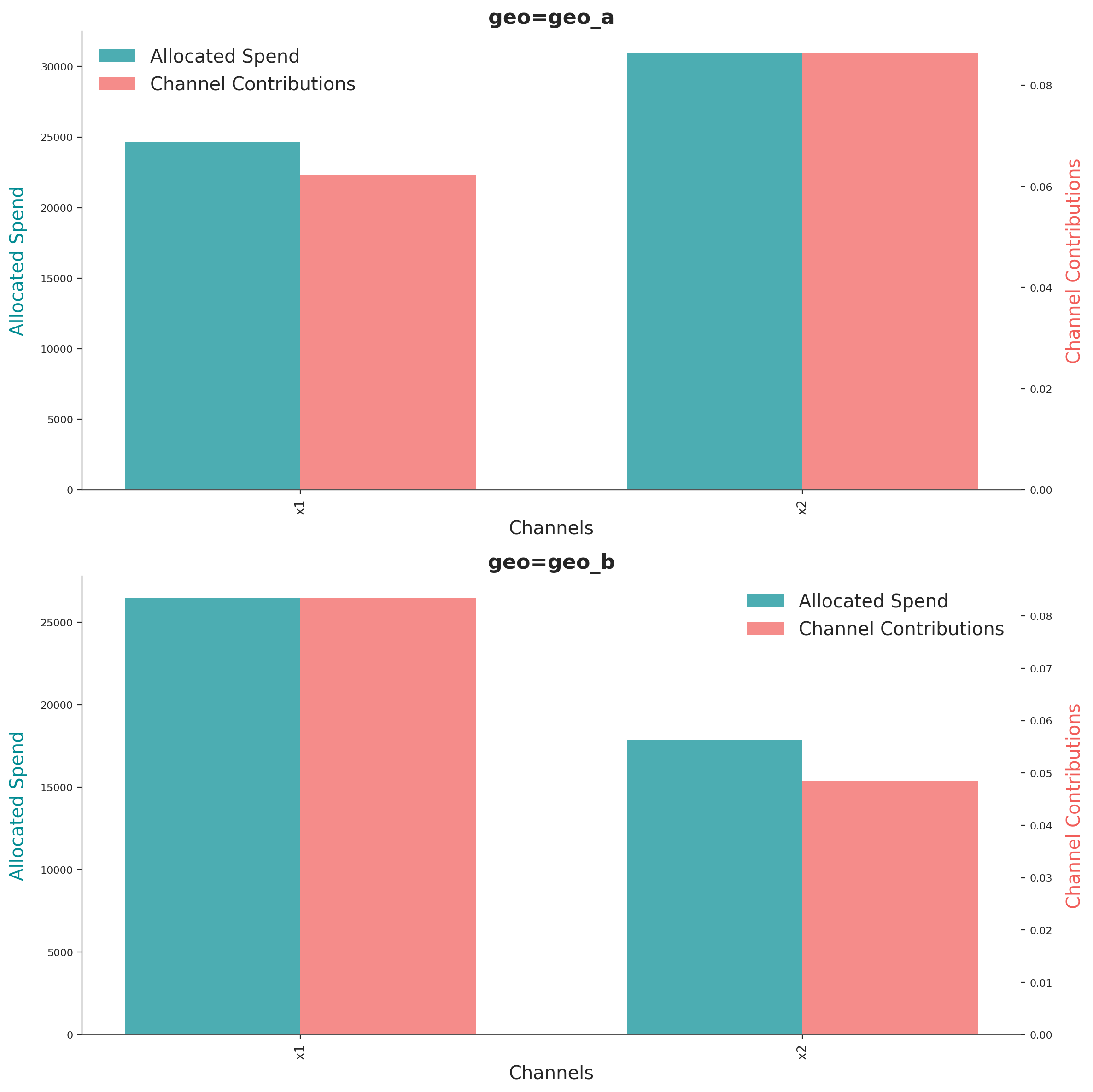
The graph shows the optimal budget for each channel on each geo, next to their respective mean contribution given the optimal budget. The method identify automatically the number of dimensions and tries to create a plot based on them.
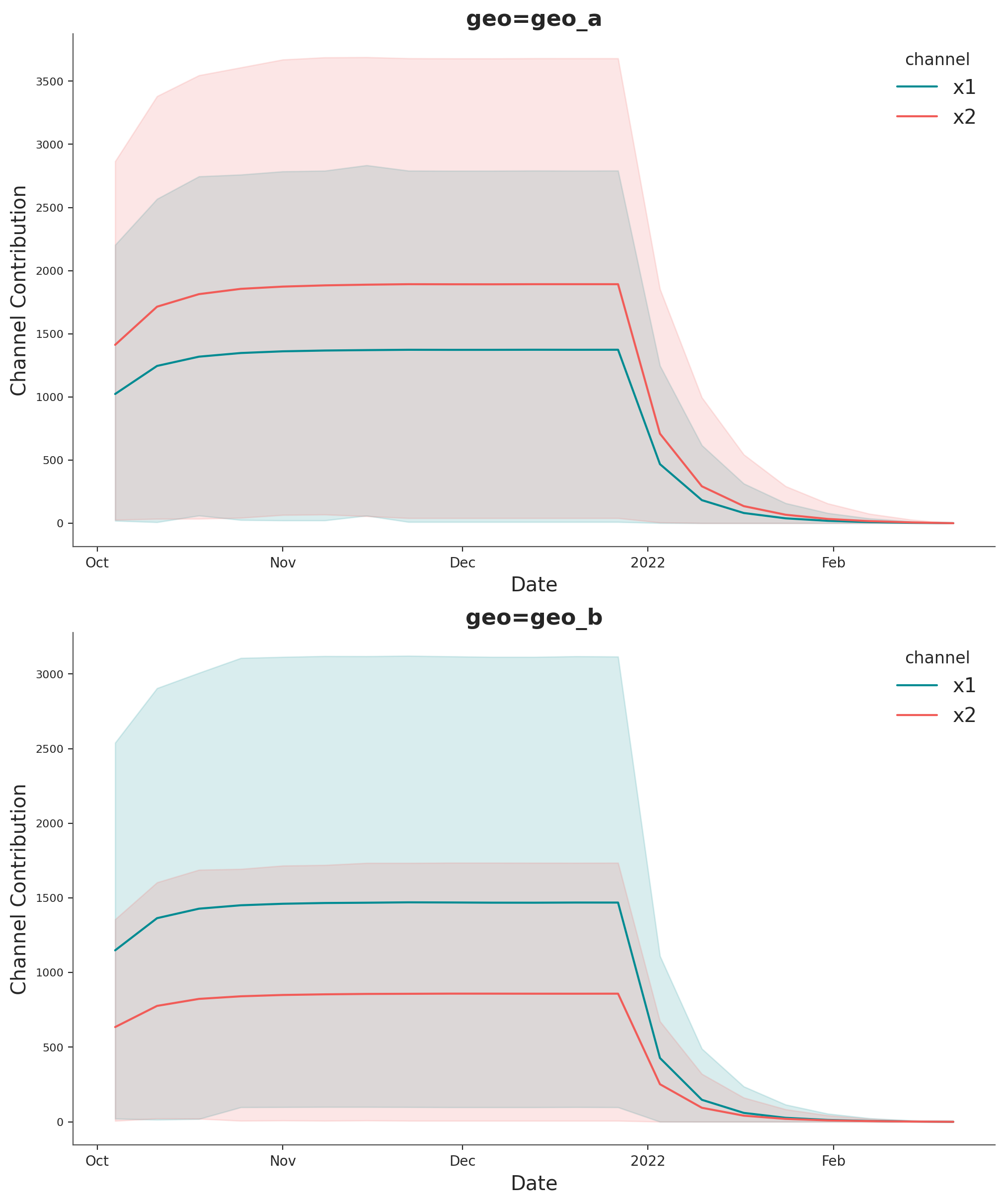
If you want to see the full uncertainty over time, you can use the plot suite and the method allocated_contribution_by_channel_over_time.
optimizable_model.plot.allocated_contribution_by_channel_over_time(
    samples=sample_allocation,
);
If you have a custom model, you can wrapped it into the model protocol, and use the optimizer after. If your model handle scales internally, you don’t need to modify anything. Otherwise, for the plots, you may want to use scale_factor=N. E.g:
optimizable_model.plot.budget_allocation(
    samples=sample_allocation,
    scale_factor=120
);
Save Model#
You can optionally save the result of your hard work. The model result objects (idata) can get very large once we start working in multiple dimensions. So it can sometimes be helpful to compress the idata before saving. Below are a couple of tricks.
# Reduce your posterior (optional)
# clone_idata = mmm.idata.copy()
# clone_idata.posterior = clone_idata.posterior.astype(np.float32)
# clone_idata.posterior = clone_idata.posterior.sel(draw=slice(None, None, 10))

# clone_idata.to_netcdf("multidimensional_model_compressed.nc", groups=["posterior", "fit_data"], engine="h5netcdf")
Note
We are very excited about this new feature and the possibilities it opens up. We are looking forward to hearing your feedback!
%load_ext watermark
%watermark -n -u -v -iv -w -p pymc_marketing,pytensor,nutpie
Last updated: Tue, 09 Jun 2026

Python implementation: CPython
Python version       : 3.13.2
IPython version      : 9.14.0

pymc_marketing: 1.0.0.dev0
pytensor      : 3.0.4
nutpie        : 0.16.10

arviz         : 1.1.0
arviz_plots   : 1.1.0
matplotlib    : 3.10.9
numpy         : 2.4.6
pandas        : 2.3.3
polars        : 1.41.2
pymc          : 6.0.1
pymc_extras   : 0.11.1.dev1+gd3254d131
pymc_marketing: 1.0.0.dev0
seaborn       : 0.13.2
xarray        : 2026.4.0

Watermark: 2.6.0